This guide walks through real training and validation loss behavior in Amazon SageMaker using XGBoost, helping you understand overfitting with a practical example.
When you train a machine learning model in Amazon SageMaker, the first thing you usually look at is the loss. If it’s going down, it feels like everything is working. But that’s not always true.
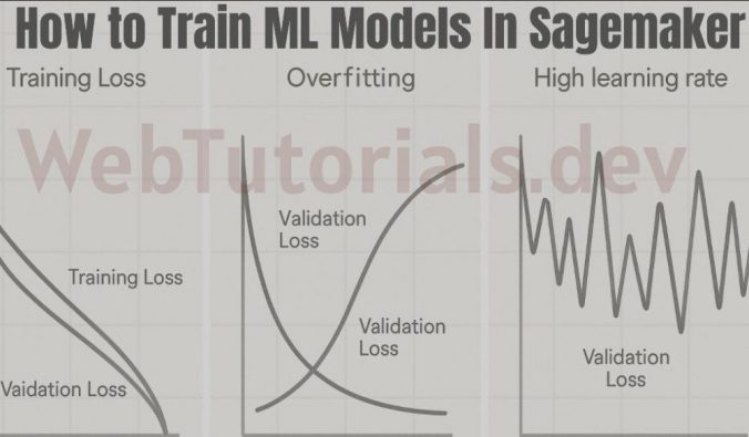
A model can show near-perfect training loss and still perform poorly on new data. The difference comes down to how you read training vs validation loss, and more importantly, the patterns between them.
If you’re trying to connect this with model evaluation, it helps to understand metrics like precision and recall first — covered here: Precision Recall F1 and AUC ROC Explained AWS MLA
In this hands-on lab, we train an XGBoost model on a simple loan approval dataset and run two controlled experiments:
- one that produces healthy training behavior
- one that clearly shows overfitting
By keeping the data constant and only changing hyperparameters, you’ll see how small configuration changes can completely alter model behavior.
Instead of relying on theory, this walkthrough focuses on what actually matters in practice:
- how loss evolves during training
- how to spot overfitting early
- and how to interpret SageMaker training logs correctly
If you’ve ever wondered why a model that “looked good” during training fails later, this will make it obvious.
- Environment Setup (SageMaker Studio)
- What We Built
- Step 1: Setup
- Step 2: Create Loan Dataset (2000 rows)
- Step 3: Split & Upload to S3
- Step 4: Training Helper Function
- Step 5: Experiment 1 — Healthy Baseline
- Step 6: Experiment 2 — Overfitting
- Step 7: Plot Both Side by Side
- Hyperparameter Comparison
- Key Takeaways
- Final takeaway
Environment Setup (SageMaker Studio)
Before running the code, here’s exactly how the environment was created in SageMaker:
- Go to SageMaker AI → SageMaker Studio
- Select JupyterLab (Private)
- Create a new JupyterLab space
- Choose instance type:
ml.t3.medium(General Purpose)
- Start the space and click Run Space
- Once status is Running, click Open JupyterLab
- Under Notebook options, select:
- Python 3 (ipykernel)
This setup is lightweight, cost-effective, and sufficient for running XGBoost experiments.
What We Built
Trained XGBoost on a loan approval dataset (2000 applications) with two different hyperparameter settings to visually see the difference between healthy training and overfitting.
Step 1: Setup
import boto3
import sagemaker
import pandas as pd
import numpy as np

from sagemaker import image_uris
from sagemaker.estimator import Estimator
from sklearn.datasets import make_classification
from sklearn.model_selection import train_test_split

session = sagemaker.Session()
region = boto3.Session().region_name
role = sagemaker.get_execution_role()

bucket = session.default_bucket()
prefix = "loss-patterns-xgboost"
Output:
Region: us-east-1
Bucket: sagemaker-us-east-1-<YOUR_ACCT_NUMBER>
Role: arn:aws:iam::<YOUR_ACCT_NUMBER>:role/service-role/AmazonSageMaker-ExecutionRole-20260107T210386
Step 2: Create Loan Dataset (2000 rows)
np.random.seed(42)
n = 2000

age = np.random.randint(21, 65, n)
annual_income = np.random.randint(20000, 120000, n)
debt = np.random.randint(0, 40000, n)

# The "rule": approved if income-to-debt ratio is good + some randomness
score = (annual_income / 1000) - (debt / 500) + (age / 10)
noise = np.random.normal(0, 10, n)
approved = (score + noise > 50).astype(int)

big_df = pd.DataFrame({
    "approved": approved,
    "age": age,
    "annual_income": annual_income,
    "debt": debt
})

print(big_df.head(10))
print(f"\nTotal: {len(big_df)}, Approved: {approved.sum()}, Rejected: {n - approved.sum()}")
Output:
   approved  age  annual_income   debt
0         0   59          45426  19029
1         0   49          37772  22973
2         0   35          23712  39121
3         0   63          21367  31433
4         1   28         111736   1932
5         0   41          71924   1757
6         0   59          23726  30722
7         0   39         109152  37853
8         0   43          47723  38405
9         0   31          29108   1116

Total: 2000, Approved: 669, Rejected: 1331
The pattern: Higher income + lower debt = more likely approved.
Step 3: Split & Upload to S3
from sklearn.model_selection import train_test_split

train_df, val_df = train_test_split(big_df, test_size=0.2, random_state=42, stratify=approved)

train_path = "/tmp/loan_train.csv"
val_path = "/tmp/loan_val.csv"

train_df.to_csv(train_path, header=False, index=False)
val_df.to_csv(val_path, header=False, index=False)

prefix2 = "loan-loss-patterns"
train_s3_loan = session.upload_data(train_path, bucket=bucket, key_prefix=f"{prefix2}/train")
val_s3_loan = session.upload_data(val_path, bucket=bucket, key_prefix=f"{prefix2}/validation")

print(f"Train: {train_df.shape}, Val: {val_df.shape}")
Output:
Train: (1600, 4), Val: (400, 4)
Train S3: s3://sagemaker-us-east-1-<YOUR_ACCT_NUMBER>/loan-loss-patterns/train/loan_train.csv
Val S3: s3://sagemaker-us-east-1-<YOUR_ACCT_NUMBER>/loan-loss-patterns/validation/loan_val.csv
- 1600 rows for training (the textbook)
- 400 rows for validation (the exam)
stratify=approvedkeeps distribution consistent
Step 4: Training Helper Function
from sagemaker import image_uris

container = image_uris.retrieve(
    framework="xgboost",
    region=region,
    version="1.7-1",
    py_version="py3",
    instance_type="ml.m5.large",
)

def train_loan(job_name_suffix, hyperparameters):
    estimator = Estimator(
        image_uri=container,
        role=role,
        instance_count=1,
        instance_type="ml.m5.large",
        output_path=f"s3://{bucket}/{prefix2}/output",
        sagemaker_session=session,
        base_job_name=f"loan-{job_name_suffix}",
        enable_sagemaker_metrics=True,
    )
    estimator.set_hyperparameters(
        objective="binary:logistic",
        eval_metric="logloss",
        num_round=hyperparameters["num_round"],
        eta=hyperparameters["eta"],
        max_depth=hyperparameters["max_depth"],
        min_child_weight=hyperparameters["min_child_weight"],
        subsample=hyperparameters["subsample"],
        colsample_bytree=hyperparameters["colsample_bytree"],
    )
    estimator.fit(
        {
            "train": sagemaker.inputs.TrainingInput(train_s3_loan, content_type="text/csv"),
            "validation": sagemaker.inputs.TrainingInput(val_s3_loan, content_type="text/csv"),
        },
        wait=True,
        logs=True,
    )
    return estimator
Step 5: Experiment 1 — Healthy Baseline
loan_baseline = train_loan("baseline", {
    "num_round": 80,
    "eta": 0.1,
    "max_depth": 4,
    "min_child_weight": 3,
    "subsample": 0.8,
    "colsample_bytree": 0.8,
})
Output (truncated)
[0]  train-logloss:0.66437  validation-logloss:0.66714  → "I know nothing"
[20] train-logloss:0.25679  validation-logloss:0.27359  → "Learning the pattern"
[50] train-logloss:0.14704  validation-logloss:0.17430  → "Getting good"
[79] train-logloss:0.11584  validation-logloss:0.15662  → "Learned it"
Result:
Training loss ↓
Validation loss ↓
Small gap between them → Healthy model ✅
Step 6: Experiment 2 — Overfitting
loan_overfit = train_loan("overfit", {
    "num_round": 400,
    "eta": 0.2,
    "max_depth": 10,
    "min_child_weight": 1,
    "subsample": 1.0,
    "colsample_bytree": 1.0,
})
Output (truncated)
[0]   train-logloss:0.xxx   validation-logloss:0.xxx   → Both start high
[50]  train-logloss:low     validation-logloss:low      → Both dropping (looks good so far)
[200] train-logloss:tiny    validation-logloss:going UP  → OVERFITTING STARTS
[399] train-logloss:0.00779 validation-logloss:0.25242  → Memorized training, failing validation
Result:
Training loss → near zero
Validation loss → increases
Result: Train loss near zero, validation loss HIGH and rising ❌ Overfitting
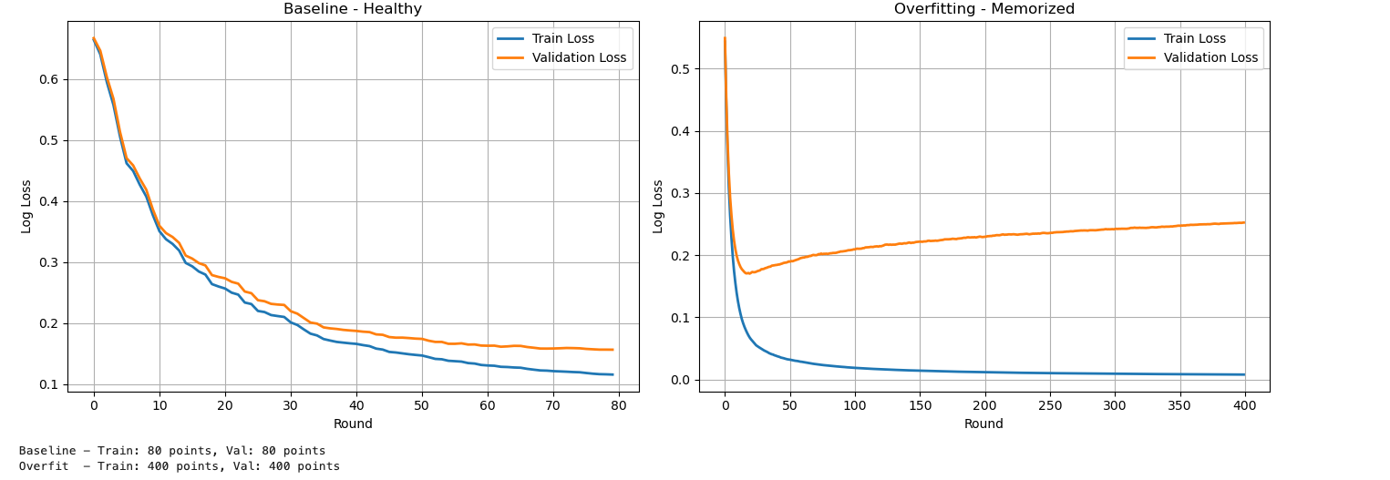
Step 7: Plot Both Side by Side
import boto3
import re
import matplotlib.pyplot as plt
from sagemaker.analytics import TrainingJobAnalytics

logs_client = boto3.client("logs", region_name=region)

def get_loss_from_logs(estimator):
    job_name = estimator.latest_training_job.name
    log_group = "/aws/sagemaker/TrainingJobs"

    streams = logs_client.describe_log_streams(
        logGroupName=log_group,
        logStreamNamePrefix=job_name + "/algo"
    )
    stream_name = streams["logStreams"][0]["logStreamName"]

    events = logs_client.get_log_events(
        logGroupName=log_group,
        logStreamName=stream_name,
        startFromHead=True,
        limit=500
    )

    train_loss = []
    val_loss = []
    for event in events["events"]:
        msg = event["message"]
        if "train-logloss" in msg and "validation-logloss" in msg:
            train_match = re.search(r"train-logloss:([\d.]+)", msg)
            val_match = re.search(r"validation-logloss:([\d.]+)", msg)
            if train_match and val_match:
                train_loss.append(float(train_match.group(1)))
                val_loss.append(float(val_match.group(1)))
    return train_loss, val_loss

train_b, val_b = get_loss_from_logs(loan_baseline)
train_o, val_o = get_loss_from_logs(loan_overfit)

fig, axes = plt.subplots(1, 2, figsize=(14, 5))

axes[0].plot(train_b, label="Train Loss", linewidth=2)
axes[0].plot(val_b, label="Validation Loss", linewidth=2)
axes[0].set_title("Baseline - Healthy")
axes[0].set_xlabel("Round")
axes[0].set_ylabel("Log Loss")
axes[0].legend()
axes[0].grid(True)

axes[1].plot(train_o, label="Train Loss", linewidth=2)
axes[1].plot(val_o, label="Validation Loss", linewidth=2)
axes[1].set_title("Overfitting - Memorized")
axes[1].set_xlabel("Round")
axes[1].set_ylabel("Log Loss")
axes[1].legend()
axes[1].grid(True)

plt.tight_layout()
plt.show()
Hyperparameter Comparison
| Setting | Baseline | Overfit | Effect |
|---|---|---|---|
| num_round | 80 | 400 | More rounds → memorization |
| eta | 0.1 | 0.2 | Faster learning → less stable |
| max_depth | 4 | 10 | Deeper trees → overfit |
| min_child_weight | 3 | 1 | Easier splits → memorization |
| subsample | 0.8 | 1.0 | Less randomness |
| colsample_bytree | 0.8 | 1.0 | Uses all features |
Loss Comparison
| Model | Train Loss | Val Loss | Gap | Verdict |
|---|---|---|---|---|
| Baseline | 0.116 | 0.157 | Small | Healthy ✅ |
| Overfit | 0.007 | 0.252 | Large | Overfitting ❌ |
Key Takeaways
- Training loss alone is misleading
- Always compare training vs validation
- Small gap = generalization
- Large gap = overfitting
- Hyperparameters control behavior
- Same data can produce very different results
Final takeaway
Most model issues are not caused by bad data — they come from how the model is trained.
In SageMaker, you don’t need complex tools to diagnose problems.
Just watch the loss:
- If training and validation move together → good model
- If they diverge → overfitting
Once you start reading loss patterns this way, debugging models becomes much simpler.
